3.3. The Graphical User Interface (GUI) execution mode

3.3.1. Launching the GUI

The Phosphoros Graphical User Interface (GUI) provides an interactive and user-friendly execution mode. After starting Phosphoros (see Download and Installation section), the GUI can be launched by the command line:

> Phosphoros GUI

Once the GUI starts, a window opens (see Fig. 3.3). At the top of this, a navigation menu is visible with the main steps of Phosphoros: Configuration, Catalog Types, Parameter Space, Compute Redshifts and Post Processing. The menu is visible at all times, and it allows you to navigate through the different Phosphoros panels.

Fig. 3.3 Starting window of the Phosphoros GUI

3.3.2. GUI: Configuration

Configuration allows users to see, and eventually to change, the default directory configuration, and to check the available auxiliary data present in the Phosphoros database. Three sub-panel can be opened:

• General Here the Phosphoros root path is shown, along with the default directories for input/output data. No changes are required if users keep the standard directory structure. Otherwise, the path to new directories can be selected through the Browse tabs.

  Users can choose the number of sources to keep in memory simultaneously (the default value is 5000): high values will speed up the execution of the template fitting, at the expense of increasing the memory usage. Users can also fix a cap in the memory usage by clicking on the Template Fitting: Cap the memory usage button and selecting the maximum value (see Fig. 3.4). This is a further way to limit the number of sources in memory. Moreover, it is possible to choose the number of unit of execution (or thread) within a process, by clicking on the Override the Maximum Number of Threads button. Otherwise, the maximum number of available threads is automatically selected.

  Finally, through Log Level drop down menu users can select logs information to be printed in the terminal when the Phosphoros GUI is running.

  

  Fig. 3.4 The Configuration: General panel of the GUI

• Auxiliary Data The Phosphoros GUI can be used to display auxiliary data files. This is not yet the place for selecting filters or SEDs (this is done in Parameter Space Definition), but it provides a view of all available auxiliary data (if any).

  The Reload Last Data Pack tab allows users to (re-)download the last available version of the auxiliary data pack from the Phosphoros repository (containing, i.e., SEDs, filters, Reddening curves, etc.). This is useful if users altered the data locally and they want to replace them with the current data pack on the repository. Close to it, there is the tab to download the Planck dust reddening map. This is needed for the Galactic absorption correction if color excess is not provided in the source catalog.

  As an example, the screenshot of Fig. 3.5 shows a possible case for the SEDs. Similarly auxiliary files in Filter Transmissions, Reddening Curves and Luminosity Function Curves can be displayed.

  In the SEDs panel, emission lines can be added to a group of SED templates by clicking on the Add Emission Line to SEDs tab associated with it. A new directory (named as the original with the postfix _el) is generated with SEDs including emission lines, without modifying the original templates (see the Emission Lines section for more details).

  

  Fig. 3.5 Example of the Configuration panel of the GUI showing SEDs present in the database

  The Import Folder tab opens a finder window and allows users to import a directory with its entire content to the location of the selected Auxiliary Data directory. On the other hand, Delete buttons remove the corresponding folders. This is an irreversible action, and a confirmation message will be always displayed before deleting.

  Here, users can also select the reference solar SED used to normalize SED templates (see SED Template Normalization), and create new SEDs by interpolating the existing ones (see SED interpolation).

• Cosmology The Cosmology tab displays the value of the cosmological parameters relevant for Phosphoros and allows users to change them. The default values are taken from Planck 2015 results [PlanckCollaboration16] (including lensing and external data): \(H_0=67.74\) [km/s/Mpc]; \(\Omega_M=0.3089\); \(\Omega_{\Lambda}=0.6911\).

3.3.3. GUI: Catalog Setup: Mapping filters to column names

In order to compute modeled photometry, Phosphoros needs the transmission curve of filters used for the observed photometry. The name of transmission curve files has to be connected with the corresponding photometric bands of input catalogs.

The GUI provides an easy way for mapping trasmission curves to catalog column names. The mapping operation is mandatory and is achieved in the Catalog Setup panel (see Fig. 3.6).

First of all, on the top of the window, users have to select the desired catalog type or to create a new one by clicking on the new or duplicate buttons. Each catalog type corresponds to a folder in the Catalogs directory, and duplicating or creating a new type will create a new folder.

The input catalog is selected by Select File and Import Columns (Phosphoros automatically selects a reference input file belonging to the catalog type). Moreover, the column name providing source ID must be entered through the Source ID Column drop down menu that shows all the column names in the input catalog.

Fig. 3.6 Catalog Setup panel and the filter mapping operation in the GUI

The mapping operation begins by pressing Select Filters: a window opens where the filter trsmission curves in the database can be selected. When the filter selection is completed, pressing Save closes the window and, as shown in the figure, fills automatically the Filter Transmission Curve column. Each of the Flux Column Name and Error Column Name cells now features a drop down menu (after clicking on the cell) which can be used to specify the appropriate Flux and FluxError column names.

If a catalog has some sources with missing photometry (sources that were not observed in all catalog bands), users have to provide a flag value in the Missing photometry flagged as control. By doing so, the program is instructed to skip photometry having the flag value in the flux column. The corresponding filters are then ignored in the \(\chi^2\) calculation.

Note

Missing photometry flags must be numbers. Symbolic values as NaN, NULL or INF are not accepted by Phosphoros.

Catalogs may contain sources that are not detected in one or more bands (i.e., the provided photometry is an upper limit of the flux and not the nominal flux). In this case, users have to ensure that the catalog follows the upper limit convention, i.e. photometry are considered upper limits when their errors have negative values. Upper limits are taken into account in the \(\chi^2\) calculation, as described in the Template fitting method section. In addition, users can set the Upper Limit recompute error flag to a specific negative value (e.g., -99): when Phosphoros finds a flux error that matches the upper limit flag, the error will be computed as \(flux/n\), where \(n\) is the number in the Upper limit over error ratio column of the Filter Mapping table. Users can change this number by clicking on the tabs (the default value is 3).

Users have also the ability to modify or re-calibrate error values in catalogs according to the following formula:

(3.1)\[ \sigma^2_k({\rm new}) = \alpha^2_k\,\sigma^2_k + \beta^2_k\,f^2_k + \gamma_k\,f_k\]

where \(f_k\) and \(\sigma_k\) are the original source fluxes and errors for the filter \(k\), while \(\alpha_k\), \(\beta_k\) and \(\gamma_k\) are coefficients chosen by users. Clicking on the Error re-calibration control, columns Alpha, Beta and Gamma will appear in the Filter Mapping table (see Fig. 3.7). The values in those columns will be used in the above formula. By default they are \(\alpha_k=1\), \(\beta_k=0\) and \(\gamma_k=0\) (i.e., no change in errors). The values can be changed clicking on the corresponding tabs. The value in a tab can be propagated to all filters by pressing Propagate Error Param .

Photometry can be also provided in AB magnitudes. To make Phosphoros aware of it, it is enough to set True in the From MAG column of the Filter Mapping table (the default is False). AB magnitudes will be then transformed to fluxes by Phosphoros.

Finally, users can map filters to the catalog columns that contain the filter shift (if present). This is required when flux corrections due to filter variations are taken into account in the redshift computation (see Advanced Features: Filter Variation).

Fig. 3.7 Catalog Setup panel and the error re-calibration operation in the GUI

Few optional fields are present in the top-right of the Catalog Setup panel: the column name of

• source coordinates (the right ascension RA (Deg) and declination DEC (Deg));

• the Milky Way extinction along source line of sight (MilkyWay E(B-V));

• the reference redshift (Reference Z).

The two first points are only required if the Milky Way absorption correction is applied (see Galactic Absorption section). In particular, sources coordinates are needed if the Planck Galactic dust reddening map is used for the correction. Otherwise, if the Milky Way extintion is provided in the input catalog, users have to fill just the MilkyWay E(B-V) tab.

When present in the input catalog, the reference redshift (e.g., spectroscopic redshift) is useful for the Post Processing analysis.

The mapping process is terminated by clicking on the Save middle-frame button. Please note that you can always add or remove filters after a first mapping has been completed, by going back to the Select Filters option.

After saving, the ASCII files named filter_mapping.txt and error_adjustment_param.txt are created in the following directory:

> $PHOSPHOROS_ROOT/IntermediateProducts/<Catalog Type>/

(in the previous examples, <Catalog Type> was Quickstart or Cosmos). They contain all the information present in the Filter Mapping table: in filter_mapping.txt you can find the qualified name of transmission curve files, the flux and flux error column names in the input catalog, etc.; while in error_adjustment_param.txt the values of the coefficients used in Eq. (3.1) to re-calibrate flux errors (see Filter Mapping in the File Format Reference chapter).

You can always edit these files to make corrections. Alternatively, you can create them with your favorite editor (rather than using the GUI). When launched, the GUI will automatically load any filter_mapping.txt (and error_adjustment_param.txt) file located in the appropriate directory, providing it respects the proper formatting.

Note

When you modify any of the GUI files using another editor, you always have to restart the GUI so that changes are taken into account.

Note

The mapping operation is carried out only once for all input catalogs belonging to the same catalog type.

3.3.4. GUI: Defining the model parameter space

An important step in Phosphoros is the specification of the model parameter space. Phosphoros parameters are four: redshift, restframe SED template, intrinsic color excess \(E_{(B-V)}\) and intrinsic reddening law. For each of them, a grid of values has to be provided by users. Phosphoros then computes, for each cell of the parameter space, a vector of modeled photometry, one value for each filter. This is called the grid of models. This calculation does not depend on observations and it can be achieved beforehand.

Clicking on Parameter Space, users can check the sets of parameter spaces that are already present in the Phosphoros database (Parameter Space drop down menu). They can be modified, duplicated or deleted; or a new one can be created (see Fig. 3.8).

In the following, we describe how to define a new parameter space and its specifications. This is done for a parameter space composed of three groups of SED templates: Elliptical, Spiral and Starburst. First of all, users have to define the values of the E(B-V) and Redshift parameters in the grid. Clicking on the Configure button, users can enter the values as a comma-separated list or as a range of values (minimum, maximum value and step) through the Add Range option (see Fig. 3.8). After saving them, select New at the Sub-Spaces of the Parameter Space level, and a new pop-up window opens, similar to that displayed in the left panel of Fig. 3.9.

Through this window, you have to provide the name of a sub-space (Elliptical, for example) and specify the SED, Reddening Curve, E(B-V) and Redshift parameters. The SED and Reddening Curve panels simply allow to select a sub-set of the data available on the system. For the E(B-V) and Redshift parameters, users can only modify the minimum and the maximum value of the ranges previously defined in Configure. Saving them, the parameter space of the (Elliptical) sub-space will be shown in the GUI panel (see Fig. 3.9).

Note

With the GUI, all sub-spaces have by default the same sampling for the E(B-V) and Redshift parameters. Users are only allowed to select out some values at the beginning or at the end of the parameter ranges. On the contrary, with the CLI, users can define different samplings for E(B-V) and Redshift in different sub-spaces (see CLI: Generating the grid of models).

The operation is terminated clicking on the Save button (at the top-right of the window). Make sure to complete the full specification of the three groups before continuing to the next section.

Fig. 3.8 Setting E(B-V) and Redshift range in the GUI

Fig. 3.9 Setting a parameter space in the GUI

3.3.5. GUI: Generating the model grid

Previous sections described how to set up Phosphoros database. In the Compute Redshifts panel, instead, Phosphoros executables are run in order to compute the grid of models and to estimate photometric redshifts.

At the top of the Compute Redshifts panel, users can select previously defined catalog types and parameter spaces to use in the following analysis.

Fig. 3.10 How to generate a grid of models in the GUI

The panel is organized into six successive sub-panels (see Fig. 3.10). The first two concern the model grid generation (1. Luminosity Filter and Extrinsic Absorption and 2. Grids Generation). Sub-panels 3–5 (3. Prior, 4. Photometric Zero-Point Corrections and 5. Algorithm) are optional functionalities and are described in the Advanced Features section. Finally, the sixth sub-panel (6. Input/Output) sets up the input and output files.

Note

Sub-panels title can be black, orange or red. The orange/red color in one of the six steps means that some actions are required before Phosphoros could run to compute redshifts. For example, if 2. Grids Generation is orange, no model grids have been produced for the selected specification yet. After the grid calculation is completed, the color turns to black indicating that the values have been computed and stored in a file that can be read in the subsequent steps of the analysis. The red color of 2. Grids Generation means that model grid and Galactic correction grid are incompatible with each other.

If you change anything in the specifications, the colour turns to orange again reminding that a new grid must be generated before continuing the analysis.

In order to produce a grid of models users have to go through with two steps:

• Luminosity Filter and Extrinsic Absorption

  In the first sub-panel, users can select:

  1) the reference filter used for the SED normalization (a default one is proposed by Phosphoros);

  2) the prescriptions for the intergalactic medium (IGM) absorption correction – Madau, Meiksin, Inoue – or OFF, if no correction is applied (see the Intergalactic medium absorption explanation).

  3) if the Milky Way absorption correction is applied or not. There are two options for the correction (see also the Galactic absorption section). The first one (Look-up Galactic E(B-V) in Planck Dust Map) fetches the Galactic color excess \(E(B-V)\) from the Planck dust reddening map. The column name of source coordinates must have been provided in the Catalog Setup panel, and the Planck map be previously dowloaded in the Configuration --> Aux.Data panel. Otherwise, Galactic color excess values can be read from the input catalog (Use Galactic E(B-V) Column). In this case, users must have provided the corresponding column name in the Catalog Setup panel. If the required information is not given, the previous options are not available to users.

  Warning

  In the case the color excess is read from the input catalog, Phosphoros assumes that those values have been derived using mean sequence B5 stars. If not, they should be scaled by the band-pass correction (see the Galactic Absorption section). This operation can be only done in the CLI mode.

  Note

  The IGM absorption correction is applied to SED templates before computing modeled photometry. On the contrary, for the Milky Way absorption, correction coefficients are applied directly to modeled photometry, i.e. after computing the grid of models (see the Galactic absorption section).

• Grids Generation

  In order to generate the grid of models, users have to specify a filename for storing the output. By default, a filename is automatically generated concatenating Grid with the parameter space name and the selected IGM prescription (e.g., Grid_<parameter space name>_MADAU). The output file is stored in the following directory:

  > $PHOSPHOROS_ROOT/IntermediateProducts/<Catalog Type>/ModelGrids/
  

  Clicking on the (Re)-Generate the Grid button generates the grid of models, while on Save Config. File a configuration file with all the command line options needed to generate the grid of models with the CLI is saved.

  If the Milky Way absorption correction has been selected in the previous step, the grid of correction coefficients has to be generated using the corresponding (Re)-Generate the Grid button. The coefficients grid file is stored in the directory:

  > $PHOSPHOROS_ROOT/IntermediateProducts/<Catalog Type>/GalacticCorrectionCoefficientGrids/
  

  The default name follows the model grid name plus _MW_Param. As before, click on Save Config. File to store the configuration file.

  Finally, if the Filter Shift button has been activated in the Catalog Setup panel (see Advanced Features: Filter variation), the grid of filter variation correction coefficients has to be generated with the Filter Variation Correction Grid File button. The file is stored in:

  > $PHOSPHOROS_ROOT/IntermediateProducts/<Catalog Type>/FilterVariationCoefficientGrids/
  

  with the default name that is the model grid name plus _FS_Param.

3.3.6. GUI: Computing Redshifts

The sub-panel six, 6. Input/Output, is the last step before estimating the best-fit model and the photometric redshift for input sources. Here, users have to specify the input catalog to analyze and the outputs to be generated by Phosphoros (Fig. 3.11).

Note

So far, users were not required to specify any input catalog. Previous steps in fact need to know only the catalog type which the input catalog belongs to.

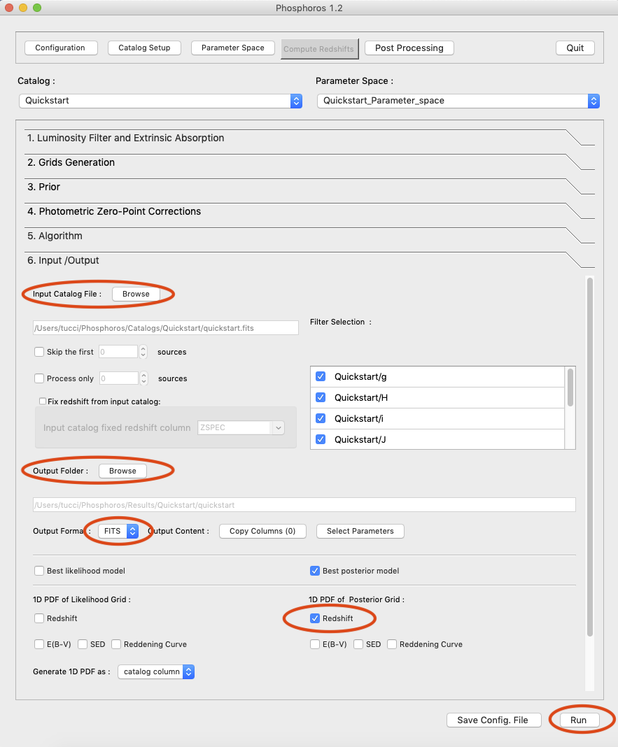
Fig. 3.11 Setting input/output of Phosphoros for the redshift computation in the GUI

Users need to fill the following information:

• Input Catalog

  As input catalog Phosphoros selects the catalog provided in the Catalog Setup panel. Different choices can be done using the Browse tab, as long as they belong to the Catalog Type defined above.

  Users can decide to run Phosphoros on a reduced number of input sources, by skipping the first or last N objects (through the Skip the first or Process only buttons).

  On the right side, Filter Selection allows users to disable some of the previously selected filters. This is useful if users want to performed particular analyses with a reduce set of photometric bands.

  Checking on Fix Redshift from input catalog, Phosphoros can also run with fixed redshifts, i.e. on a catalog where redshift is known for all sources, for example from spectroscopy. This can be useful to derive, for example, the source best fit SED and/or physical properties such as age, star-formation rate etc. The input catalog column containing the reference redshifts has to be selected from the Input catalog fixed redshift column drop-down menu.

• Output catalog

  Phosphoros results are stored in an output file named phz_cat that is by default located into:

  > $PHOSPHOROS_ROOT/Results/<Catalog Type>/<Catalog File Name>/
  

  where the Catalog File Name is the name of the input catalog file without the extension. Users can however choose another location by clicking on the Browse button. The output catalog can be saved either in FITS or in ASCII format.

  Columns from the input catalog can be also copied into the output catalog (Output Content). The Copy Columns (0) tab indicates that no input columns are selected. Click on it and a window will appear with the list of all input catalog columns. Select columns to be copied. The number in the Copy Columns tab will be updated.

  Users can include in the output catalog the best-fit model parameters from the likelihood or posterior distribution or from both, selecting Best likelihood model and/or Best posterior model.

  Typical ouput catalogs include the following information (see File format reference section for more details on output files):

  • the source ID,

  • the best model (\(z\), SED, E(B-V), reddening cuve) from the likelihood and/or posterior distribution,

  • the amplitude of the likelihood and/or posterior distribution for the best-fit model,

  • the normalized scale factor \(\alpha\) for the best-fit model,

  • the redshift value at the peak of the redshift PDF.

• (Optional) 1D PDF

  1D PDF of model parameters (from the likelihood and/or the posterior distribution) can be computed and stored for each source by selecting the desired parameters. Using the Generate 1D PDF as tab, 1D PDFs can be saved as columns of the output catalog (containing vector data) or as individual FITS files, one per parameter (see File format reference section).

  In the GUI, 1D PDFs from a likelihood are generated by a Maximum Likelihood method, while 1D PDFs from a posterior distribution by Marginalization of the other model parameters (see Axis Collapse options for more details).

• (Optional) Multi-Dimensional Output

  Users can enable the generation of FITS files containing the full posterior distribution, one per source (the Full grid option in the Multi-Dimensional Output menu). This action will produce a large volume of data (see File format: Outputs). Otherwise, in order to reduce the dimension of output files, users can save only a sampling of posterior distributions by selecting Sampling and choosing the Sample number (default 1000). In this case, Phosphoros stores the parameter values for the sampled models, whose density in the parameter space gives the posterior probability (e.g., the 1D PDF of a model parameter can be simply obtained from the histogram of its values).

  Multi-dimensional outputs can be investigated using the appropriate Phosphoros tool in the CLI (see Posterior Investigation).

  Note

  The full posterior distribution is computed after the marginalization of the scale factor (if it is not fixed to its best-likelihood value).

After setting Input/Ouput, users are ready to start the computation of photometric redshifts, clicking on the Run button. All results are written into the Output Folder defined above.

Note

Users do not need to go through all the points above. Select just the ones you need. If the Run button is inactive, it means that something is not setup yet and the computing can not be done. In such case, just hover the mouse pointer on the button and a tool tip will apears with a list of the missing steps.

The button Save Config. File exports the settings of the different actions used for the redshift computation into configuration files (e.g., ModelGrid.CMG.conf, GalacticCorrGrid.CGCCG.conf, TemplateFitting.CR.conf, etc.). They are located in a directory choosen by the user (by default $PHOSPHOROS_ROOT/config/). A file, named command, is also generated with the list of the Phosphoros commands needed to repeat the GUI run using the CLI.

PlanckCollaboration16

Planck Collaboration. Planck 2015 results. XIII. Cosmological parameters. A&A, 594:A13, Sep 2016. arXiv:1502.01589, doi:10.1051/0004-6361/201525830.