5. Methodology

This section aims to describe the main operations developed by the Phosphoros algorithm and to provide the methodology background required to better understand all the Phosphoros steps. A more detailed explanation about the formalism, assumptions and input data used in Phosphoros can be found in the Phosphoros paper []. This section is complementary to the previous Basic Steps and Advanced Features sections, which are focused on how to execute Phosphoros in the GUI and in the CLI.

5.1. Templates

Phosphoros requires a library of restframe spectral energy distribution (SED) templates as input. Templates can be empirical (typically from spectroscopic observations of nearby galaxies), synthetic (from stellar population models), or a mix of both. The library can also comprise SEDs of galaxies with a potential contribution of active galactic nuclei (AGN) as well as star templates. It is left up to users to create a less or more complex template library.

The Phosphoros data repository includes a set of commonly used templates for galaxies, AGN, AGN-host galaxies and stars. A detailed description of the Phosphoros library is given in the Data Repository (under construction) chapter. It contains, for example, the COSMOS template library (Ilbert et al. 2009 []), shown in Fig. 5.1.

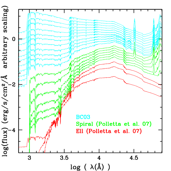
Fig. 5.1 The 31 SED templates from the COSMOS library (figure from Ilbert et al. 2009): it includes seven templates for elliptical galaxies (from E1 to E7; red curves); twelve for spiral galaxies (from S0 to Sdm; green curves); twelve for young blue star-forming galaxies (from SB0 to SB11; cyan curves). The flux scale is arbritary.

Note

The only requirement for input spectra is to follow the standardized format described in File Format: Input files.

5.2. Intrinsic interstellar dust absorption

SED templates of extragalactic sources have to be modified in order to take into account the effects of extinction due to intrinsic interstellar dust. After extinction, the source flux \(f_{ext}\) at the restframe wavelength \(\lambda\) is attenuated by

\[f_{ext}(\lambda)=f_{int}(\lambda)\times 10^{-0.4k(\lambda)E_{B-V}}\,,\]

where \(f_{int}\) is the intrinsic flux and \(k(\lambda)\) is the attenuation curve (or reddening curve; see Fig. 5.2) that defines the dependence of absorption with wavelength. The color excess \(E_{B-V}\) controls the overall amount of absorption. Both the reddening curve and the color excess are free parameters in the grid of models (see Basic Steps: Generating the model grid).

Commonly adopted reddening curves are provided as auxiliary data in Phosphoros (see the Data Repository (under construction) chapter): e.g., the Calzetti et al. (2000 []) dust law for starburst galaxies; the Fitzpatrick (1986 []) law for the Large Magellanic Cloud; the Prevot et al. (1984 []) law for the Small Magellanic Cloud. Users can add and adopt different attenuation prescriptions.

Fig. 5.2 Examples of reddening curves (figure from Cao et al. 2018 []).

5.3. Intergalactic medium absorption

The SED of sources at cosmological distances are also attenuated by absorption due to the intergalactic medium (IGM) between observer and source. This absorption is mainly due to the neutral hydrogen contained in discrete clouds of primordial gas located along the line of sight at various redshifts. It affects the source flux at wavelengths shortward of \({\rm Ly}\alpha\) (i.e., 1216\(\mathring{\rm A}\) at the emitter restframe).

Common prescriptions from literature provide an estimate of the mean effective IGM optical depth, \(\tau_{eff}\), along the line of sight of a source. They are in fact based on estimates of the average density and chemical properties of absorbers in the Universe. The IGM impact on the source flux at restframe wavelength \(\lambda\) is evaluated as:

\[f_{ext,IGM}(\lambda)=f_{ext}(\lambda)\times e^{-\tau_{eff}(\lambda,z)}\,.\]

The effective optical depth \(\tau_{eff}\) depends on the restframe wavelength, modifying consequently the shape of the SED. It depends also on the source redshift since the absorbers’ column density increases with distance. The IGM attenuation is computed for each redshift of the grid of models.

Three different prescriptions are currently implemented in Phosphoros in order to compute the effective optical depth (see Fig. 5.3).

1. Madau 1995 []: the most commonly adopted prescription in template-fitting codes for photometric redshifts. It assumes a Poisson distribution of absorption systems. The recipe used in Phosphoros extends the Madau prescription taking into account the Lyman series up to \(n=18\) (using the coefficients from NASA’s HEASARC 1) and metal lines. It also assumes \(\exp(-\tau_{eff})=0\) at \(\lambda < 912\)\(\mathring{\rm A}\).

2. Inoue et al. 2014 []: an update of the Madau model based on more recent observations of the intergalactic absorbers distribution. The implemented prescription follows the analytic models provided in their section 4, that approximates the Lyman series (up to \(n=40\)) and Lyman continuum absorption.

3. Meiksin 2006 []: he estimates the IGM absorption based on numerical simulations. In particular, Phosphoros considers the Meiksin prescription of the Lyman series absorption (up to \(n=31\)) and of the photoelectric absorption from optically thin and Lyman Limit systems.

Note

Because in the Inoue et al. and Meiksin formalism the value of \(\exp(-\tau_{eff})\) rises to infinity towards \(\lambda=0\), the minimum value of \(\exp(-\tau_{eff})\) is adopted at all wavelengths shorter than the wavelength corresponding to that minimum.

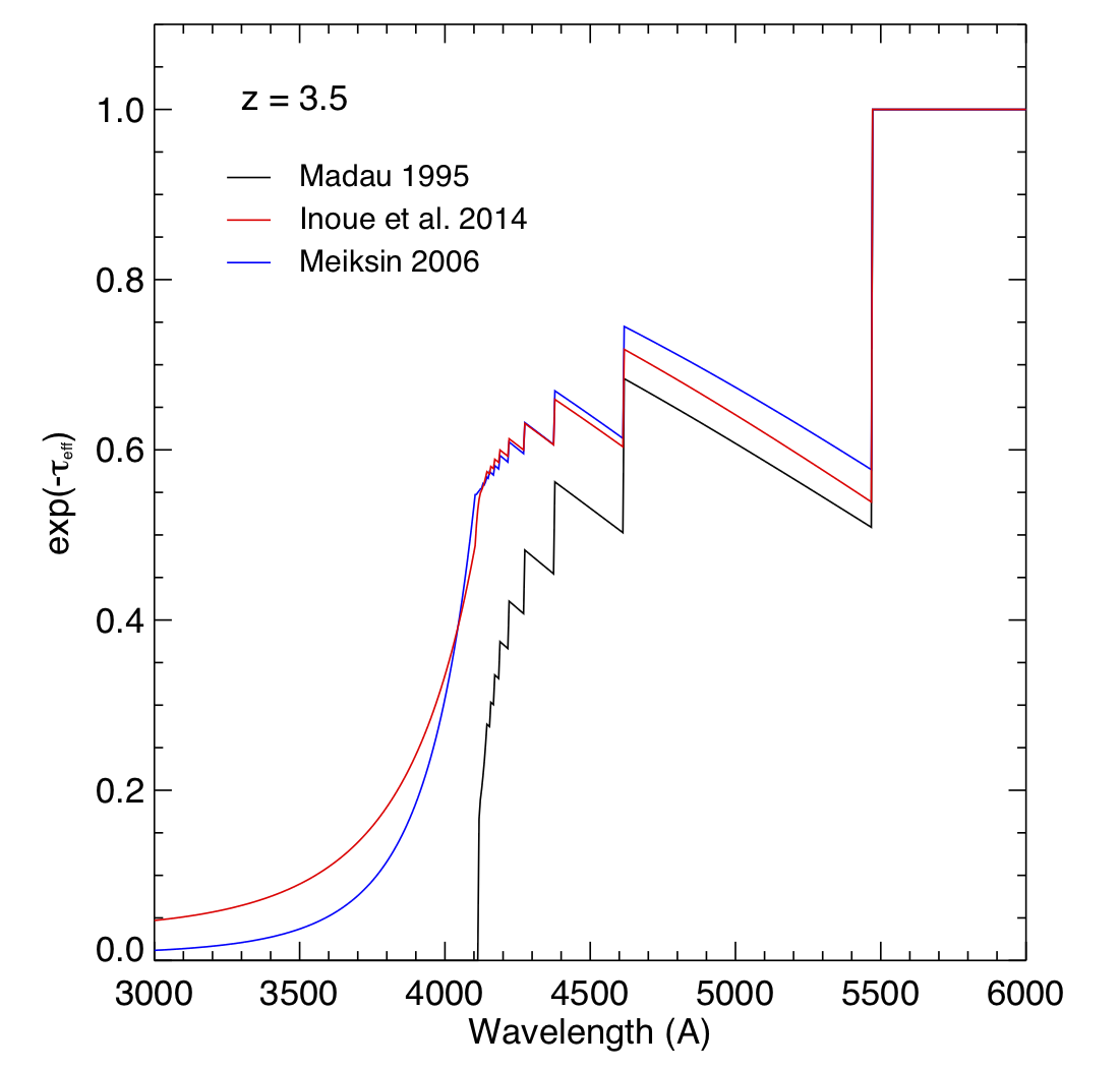
Fig. 5.3 The \(\exp(-\tau_{eff})\) curves at \(z=3.5\) for the three IGM absorption prescriptions implemented in Phosphoros.

The user can choose one of these prescriptions, but not modify them or add a new one. In Phosphoros there is also the option to not apply any IGM absorption correction. This can reduce the time to compute the grid of models when sources are expected to be at low-to-intermediate redshifts and the IGM absorption is not relevant.

Note

Photometric redshift estimates for high redshift sources significantly improve when an IGM absorption correction is applied. Phosphoros paper [] shows that photometric redshifts at \(z>2\) are biased by a factor \(\Delta z\sim0.1(1+z)\), if this correction is not taken into account. The three different prescriptions provide similar results.

Note

The current version of Phosphoros does not take into account the variability of the IGM absorption with the line of sight, which could be more or less impacted by a higher or lower number of absorbers.

5.4. Redshifting of the restframe templates

Restframe SED templates (including intrinsic and IGM absorption) are redshifted following the grid of redshifts specified by users. In particular, the wavelength is transformed from the original, restframe wavelength \(\lambda\) to one at the desired redshift, i.e. \((1+z)\lambda\). Modeled SEDs are consequently obtained as

\[f_m(\lambda)=\frac{f_{rest}(\lambda/(1+z))}{(1+z)^2}\,.\]

where the factor \(1/(1+z)^2\) takes into account the effects of redshifting on the source flux.

5.5. Applying filter trasmission curves

As a result of the above steps, a library of redshifted and attenuated SEDs is produced. In order to be compared with photometric flux measurements, modeled SEDs have to be integrated through the filter trasmission curves of the bands surveyed by the input catalog.

For photon-counting systems, such as CCDs, the observed flux through a filter \(i\) is computed by:

(5.1)\[f_m^i = \frac{\int\frac{\lambda}{c}f_m(\lambda) T_i(\lambda)d\lambda}{\int T_i(\lambda)\frac{d\lambda}{\lambda}}\,,\]

where \(T_i\) is the filter trasmission curve and \(f_m(\lambda)\) is the observer-frame modeled SED.

For energy-measuring systems, such as bolometers, the observed flux through a filter \(i\) is instead:

(5.2)\[f_m^i = \frac{\int f_m(\lambda) T_i(\lambda)d\lambda}{\int T_i(\lambda)\frac{c\,d\lambda}{\lambda^2}}\,.\]

Phosphoros is able to handle both cases, i.e. photon-counting (by default) and energy-measuring filters (see File format: Input files).

Phosphoros Data Pack repository supplies a set of filter transmission curves for the main observatories in nearIR/optical/UV bands, collected from the Filter Profile Service of the Spanish Virtual Observatory 2. For instance, Fig. 5.4 shows the filter trasmission curves used in the Euclid Data Challenge 3. Users can select the transmission curves to be used or add new ones.

Fig. 5.4 Filter trasmission curves at different bands from the Euclid Data Challenge 3.

5.6. Galactic Absorption

The observed flux of a source is also attenuated by Milky Way dust absorption. To account for Galactic absorption, Eq. (5.1) of the previous sub-section should be modified as:

(5.3)\[f^i_{m,ga} = \frac{1}{\int T_i(\lambda)\frac{d\lambda}{\lambda}} \int\,\frac{\lambda}{c} f_m(\lambda) 10^{-0.4A_{\lambda}}T_i(\lambda)d\lambda\,,\]

where \(A_{\lambda}\) is the extinction due to Milky Way absorption at wavelength \(\lambda\). This is usually expressed as \(A_{\lambda}=E^{\scriptscriptstyle MW}_{B-V}k_{\scriptscriptstyle MW}(\lambda)\), where \(k_{\scriptscriptstyle MW} (\lambda)\) is the Milky Way absorption law, normalized to the value of the color excess \(E^{\scriptscriptstyle MW}_{B-V}\). Galactic absorption, when associated with a filter, depends therefore on the source SED.

The effect of Galactic absorption is taken into account in Phosphoros after computing the grid of modeled photometry, using the following expression:

(5.4)\[f^i_{m,ga}=f^i_{m}\times 10^{-0.4A_{{\scriptscriptstyle SED},i}}\,,\]

where \(A_{{\scriptscriptstyle SED},i}\) is the total extinction for the filter \(i\) defined as the logarithmic of the ratio between the observed flux with and without Galactic absorption

(5.5)\[A_{{\scriptscriptstyle SED},i}= -2.5\log_{10}\bigg(\frac{\int_i \lambda f_m(\lambda) 10^{-0.4A_{\lambda}} T_i(\lambda)d\lambda} {\int_i \lambda f_m(\lambda)T_i(\lambda)d\lambda}\bigg) \,.\]

In the context of template-fitting codes, computing reddened SEDs by Eq. (5.5) would be too time-demanding in large catalogues. In order to include the SED dependence in the Galactic absorption correction, Phosphoros follows the prescription provided by Galametz et al. 2017 [] in their Appendix A. They show that the total extinction \(A_{{\scriptscriptstyle SED},i}\) for a given filter can be robustly approximated as a linear function of the color excess \(E^{\scriptscriptstyle MW}_{B-V}\) when \(E^{\scriptscriptstyle MW}_{B-V}\le0.3\) (i.e., for the typically values in the sky areas far from the Galactic Plane):

(5.6)\[A_{{\scriptscriptstyle SED},i}(E^{\scriptscriptstyle MW}_{B-V}) \simeq a_{{\scriptscriptstyle SED},i}\times E^{\scriptscriptstyle MW}_{B-V}\,.\]

The reddened flux can be again computed from Eq. (5.4), with \(A_{{\scriptscriptstyle SED},i}\) depending on the source SED through the parameter \(a_{{\scriptscriptstyle SED},i}\). Practically, Phosphoros will generate a grid of coefficients \(a_{{\scriptscriptstyle SED},i}\) for each different pair of {SED, filter} by computing the exact value of \(A_{{\scriptscriptstyle SED},i}\) for \(E^{\scriptscriptstyle MW}_{B-V}=0.3\) from Eq. (5.5), and setting \(a_{{\scriptscriptstyle SED},i}=A_{{\scriptscriptstyle SED},i}(0.3)/0.3\).

Note

The SED dependence of Galactic absorption is commonly neglected, and Galactic total extinction is approximated by \(A_i=E^{\scriptscriptstyle MW}_{B-V}k_{pivot}\), where \(k_{pivot}\) is the value of the Galactic absorption law at an adopted pivot wavelength \(\lambda_{pivot}\) of the filter 3. However, as discussed by Galametz et al. 2017, neglecting the SED dependence can significantly affect photometric redshifts estimates. Using a mock flux catalog of sources, they show that photometric redshifts can be biased by a factor \(\Delta z\gtrsim2-3\times10^{-3}(1+z)\) when the \(k_{pivot}\) approximation is applied. Although small, this is relevant for Euclid that requires unbiased photometric redshifts at the level of \(<2\times10^{-3}(1+z)\) []. We have verified that the Galactic absorption correction used in Phosphoros does not introduce any significant bias in photometric redshift estimates.

The Galactic absorption correction requires the knowledge of the Milky Way absorption law, \(k_{\scriptscriptstyle MW}(\lambda)\), and of the value of the color excess along the line of sight of each source. Phosphoros adopts the absorption law from Fitzpatrick 1999 [], which is calibrated using colour excesses from main sequence B5 stars, \(E^{\scriptscriptstyle B5}_{B-V}\).

Phosphoros allows two options to provide color excess values:

• the user can input the \(E^{\scriptscriptstyle MW}_{B-V}\) value associated at each source as one of the columns of the photometric catalog;

• Phosphoros can fetch \(E^{\scriptscriptstyle MW}_{B-V}\) directly from the reddening map provided by Planck [].

Warning

The absorption law \(k_{\scriptscriptstyle MW}(\lambda)\) used in Phosphoros is calibrated by main sequence B5 stars. If Galactic color excess \(E^{\scriptscriptstyle MW}_{B-V}\) is derived from different sources (e.g., Planck data use reddening measurements of quasars), \(E^{\scriptscriptstyle MW}_{B-V}\) values have to be scaled by the band-pass correction (see Galametz et al. 2017). This is a small effect and it is taken into account by Phosphoros for Planck data: in this case, the band-pass correction is \(E^{\scriptscriptstyle B5}_{B-V}=E^{\scriptscriptstyle Planck}_{B-V}\times1.018\). On the contrary, color excess from the Schlegel et al. [SchlegelFinkbeinerDavis98] Galactic reddening map does not require any band-pass correction.

Note

The Galactic absorption correction is an optional functionality in Phosphoros that can be switched off by users.

5.7. Template fitting method

As first step, Phosphoros builds a grid of modeled photometry: this consists of one photometric value for each selected filter, spanning over all possible model parameters. The parameters are: redshift \(z\), restframe SED template, color excess \(E_{B-V}\) and reddening curve \(k(\lambda)\) (the last two paramteres are related to intrinsic dust absorption).

The next step is to compute, for each source of the input catalog, the likelihood \(\mathcal{L}\) that observed photometry are described by a model \(m\). This is done via a standard \(\chi^2\) method:

(5.7)\[\ln(\mathcal{L}) = -\frac{\chi^2}{2} = -\frac{1}{2}\sum_i\bigg(\frac{f_{obs}^i-\alpha f_m^i}{\sigma_i}\bigg)^2\,.\]

The sum is over the number of selected photometric bands. \(f_{obs}^i\) and \(f_m^i\) are the observed and modeled flux for the filter \(i\), while \(\sigma_i\) is the error associated with the observed flux. The \(\chi^2\) reflects the discrepancies between the observed fluxes and a given model. The smallest \(\chi^2\) among the grid of models can therefore determine the best-fit model and consequently the photometric redshift of a source.

The normalization factor (or scale factor) \(\alpha\) present in the above equation is an additional free parameter of the model. In order to reduce the number of free parameters and to be faster, by default Phosphoros fixes \(\alpha\) to the value that minimize the \(\chi^2\). This value can be derived analytically by:

(5.8)\[\alpha = \sum_i \frac{f_{obs}^if_m^i}{\sigma_i^2} \bigg/ \sum_i \frac{(f_m^i)^2}{\sigma_i^2}\,.\]

However, in Phosphoros users have the option to sample different values of \(\alpha\) and to derive the redshift PDF after the scale factor marginalization.

Input catalogs may contain missing data, i.e. sources not imaged in one or more filters. Phosphoros simply ignores those filters in the previous formulas.

Multi-band catalogue can also include upper limits of source fluxes. This occurs when sources are not detected in one or more images due to their low fluxes. Upper limits are taken into account by Phosphoros in the \(\chi^2\) calculation following the Sawicki’s [] recipe (see their Appendix and the Phosphoros paper []) 4.

5.8. Bayesian inference and Priors

In the maximum-likelihood method, the best-fit model corresponds to the model that minimizes the \(\chi^2\). However, in many cases there are additional information, not taken into account in the likelihood, that could potentially help to have a more accurate model selection. For instance, it may be known from previous experience that one of the possible redshift/galaxy type combinations is much more likely than any other, given the galaxy magnitude.

Bayesian inference allows us to include additional information on model parameters, known a priori (priors). In this framework, the best model is estimated by finding the posterior probability distribution \(p(m|\mathbf{F}, \mathcal{P})\), i.e. the probability of a galaxy to be described by the model \(m\) given the observed photometry \(\mathbf{F}\) and the prior information \(\mathcal{P}\). Applying the Bayes’ theorem,

\[p(m|\mathbf{F}, \mathcal{P}) \propto \mathcal{L}(\mathbf{F}|m)\,\mathcal{P}(m)\,,\]

where \(\mathcal{L}(\mathbf{F}|m)\) is the likelihood previously defined in Eq. (5.7) and \(\mathcal{P}(m)\) is the prior probability distribution for a model \(m\).

For simplicity, in the following discussion, we will neglect the model parameters \(E_{B-V}\) and reddening curve. Moreover, because priors are usually known with respect to the galaxy spectral/morphological type (e.g., elliptical, spiral, starburst galaxies), we will talk about galaxy types \(T\) instead of SED templates. Hereafter, a model is just reduced to \(m=\{z,\,T\}\). The discussion can be easily extended to the rest of model parameters.

The main output of Phosphoros is the redshfit probability density function, \(PDF(z)\). In absence of priors, this is simply \(PDF(z)\equiv\mathcal{L}(\mathbf{F}|z)\); with priors, the \(PDF(z)\) is the posterior distribution for \(z\), \(PDF(z)\equiv p(z|\mathbf{F},\mathcal{P})\). This is obtained by projecting the posterior distribution to the \(z\) axis. In the reduced parameter space, it is:

\[PDF(z)\equiv p(z|\mathbf{F},\mathcal{P})=\sum_{T} p(z,T|\mathbf{F},\mathcal{P}) \propto\sum_{T}\mathcal{L}(\mathbf{F}|z,T)\,\mathcal{P}(z|T) \,\mathcal{P}(T)\,,\]

where the priors \(\mathcal{P}(T)\) and \(\mathcal{P}(z|T)\) correspond, respectively, to the fraction of \(T\)–type galaxies and their redshift distribution.

Note

Phosphoros can compute 1D probability density functions for all the model parameters, in the similar way as for the redshift PDF.

Note

As discussed above, the likelihood is typically computed by fixing the normalization factor \(\alpha\) with the value that minimizes the \(\chi^2\) for a given model. However, in a fully Bayesian approach, the template normalization \(\alpha\) should be considered as an additional model parameter. In this case, the redshift \(PDF\) is derived by marginalizing over the \(\alpha\) parameter too:

\[p(z|\mathbf{F},\mathcal{P})=\sum_{T}\int d\alpha\, p(z,T,\alpha|\mathbf{F},\mathcal{P}) \propto\sum_{T}\int d\alpha\, \mathcal{L}(\mathbf{F}|z,T,\alpha)\,\mathcal{P}(z,T)\,.\]

where we have assumed a flat prior for \(\alpha\), and that the galaxy redshift and type do not depend on \(\alpha\).

Note

In the above discussion SED templates are grouped in different types, whose priors correspond to their fractions with respect to the total family of galaxies. Phosphoros deals with the issue of the weight of each template within a galaxy type too. It assigns in fact a weight to each SED template based on the volume of the color space uniquely covered by the template (see the Phosphoros paper [] and Advanced features: SED weights for more details).

Phosphoros provides some default prior functionalities that can be applied to the likelihood of models. They consist in priors on the source luminosity, redshift distribution and volume, and they are the topic of the next sub-sections. In addition, Phosphoros allows users to introduce their own pre-computed priors on one or multiple model parameters (see Advanced features: Ganeric Prios ).

5.8.1. Redshift distribution

Prior information are often given in terms of redshift distribution for galaxies with apparent magnitude \(m_0\), i.e. \(p(z|m_0)\) (see, e.g., Benitez et al. 2000 [Benitez00]). The prior can include information such as the existence of upper or lower limits on galaxy redshifts, or discriminate values of redshifts that are considered less or more probable with respect to other ones.

Because galaxies belonging to different morphological/spectral types may have different distributions in redshift, the prior definition is usually expanded into the probability \(\mathcal{P}(z,T|m_0)\), i.e. the probability of the galaxy redshift being z and the galaxy type being T given an apparent magnitude \(m_0\). It follows that

\[\mathcal{P}(z,T|m_0)=\mathcal{P}(T|m_0)\,\mathcal{P}(z|T,m_0)\,,\]

where \(\mathcal{P}(T|m_0)\) is the galaxy type fraction as a function of magnitude, and \(\mathcal{P}(z|T,m_0)\) is the prior information on the redshift distribution for galaxies of the given type and magnitude. The redshift \(PDF\) is then expressed in terms of prior distributions as:

\[PDF(z) \propto\sum_T \mathcal{L}(\mathbf{F}|z,T)\,p(z,T|m_0) =\sum_T \mathcal{L}(\mathbf{F}|z,T)\,\mathcal{P}(T|m_0) \,\mathcal{P}(z|T,m_0)\,.\]

See the Redshift Distribution Priors section for a detailed explanation of redshift priors in Phosphoros and of their use.

5.8.2. Volume correction

Phosphoros implements the so called volume correction. This prior information takes into account the fact that a survey covers larger volumes of the Universe at higher redshift than at lower redshift, and consequently gives higher probability to find a galaxy at higher redshift. The prior distribution depends only on redshift and is given by:

\[\mathcal{P}(z)\propto \frac{dV_c}{dz} = 4\pi D_c^2\frac{dD_c}{dz}\,,\]

where \(D_c~(V_c)\) is the comoving distance (volume) at redshift \(z\).

See the Volume Prior section for its use in Phosphoros.

5.8.3. Luminosity functions

Another example of prior information implemented by Phosphoros is given by the galaxy luminosity function, \(\phi(L_b,z)\). Luminosity functions can be seen in fact as a probability function, i.e. the probability for a source to have a particular luminosity at a given redshift. Here, the luminosity \(L_b\) refers to the intrinsic luminosity (or, equivalently, the magnitude) integrated over a specific observational band \(b\).

For each model of the parameter space we can compute the luminosity in the \(b\) band, \(L_{b,m}\), and consequently, through the luminosity function, the prior probability for that model. If luminosity functions are known over the full redshift range and for all galaxy types, the redshift \(PDF\) with luminosity priors becomes:

(5.9)\[PDF(z)\equiv p(z|\mathbf{F},\mathcal{P})=\sum_{T} p(z,T|\mathbf{F},\mathcal{P})\propto\sum_{T} \mathcal{L}(\mathbf{F}|z,T)\,\phi_{z,T}(L_{b,m})\,,\]

where \(\phi_{z,T}\) is the luminosity function of \(T\)–type galaxies at redshift \(z\). In the above equation, we have assumed \(\phi_{z,T}(L_{b,m})=\mathcal{P}(z,T)\) and a uniform prior for \(\mathcal{P}(T)\).

We refer users to the Luminosity Priors section for a detailed explanation on luminosity priors in Phosphoros and their use.

Footnotes

1

see https://heasarc.gsfc.nasa.gov/xanadu/xspec/models/zigm.html

2

see https://http://svo2.cab.inta-csic.es/svo/theory/fps3/

3

A typical way to define the filter pivot wavelength is \(\lambda_{pivot}=\sqrt{\int\lambda T_i d\lambda/\int T_i d\lambda/\lambda}\), where \(T_i\) is the trasmission curve of filter \(i\).

4

Equation A10 of Sawicki et al. is modified in Phosphoros in order to avoid negative values of \(\chi^2\), replacing the factor \(\sqrt{\pi/2}\sigma_j\) in the second term of the equation by 0.5.