2. Quickstart in 15 minutes

If you have never used Phosphoros and you want to whet your appetite, this 15 minutes quickstart tutorial is intended just for you! It will give you a brief overview of the Phosphoros workflow and guide you through a simple example of computing photometric redshifts, without explaining in detail each step. At the end of the quickstart you will have an idea how it feels like to use Phosphoros.

This quickstart assumes that you have a functional version of Phosphoros already installed (version 1.3; if you do not, before you continue, you should install Phosphoros by following the instructions here) and you are ready to launch the Phosphoros Graphical User Interface (GUI).

2.1. Template fitting in two words

Phosphoros is a tool for estimating photometric redshifts using template fitting method. The method consists of two steps. During the first step, which has to be performed only once, we define a set of models, for which we compute photometry in specific wavelength bands. You can imagine models as a multi-dimensional parameter space, whose axes are SED template, redshift and reddening (color excess and extintion curve). Each point of this parameter space contains modeled photometry.

During the second step, we take the photometry of a source of unknown redshift and we compare them with our models: the likelihood for the full parameter space is computed using the \(\chi^2\) distance. Based on which models match better the observed photometries, we estimate the best-fit photometric redshift and the redshift Probability Density Function (i.e. the probability of a source to be at a given redshift).

The following sections will navigate you through the quickstart data, settings, and a basic data analysis, in order to get an idea on how each step is performed with the Phosphoros GUI.

2.2. Getting the quickstart data

All the data required to run the quickstart can be downloaded as a single tar file from the Phosphoros repository. It includes the quickstart source catalog and eight filter transmissions (plus the filter mapping file and the parameter space file for quickstart). You just have to uncompress the file in a directory called Phosphoros under your home directory. All the quickstart data will be located in the proper directories according to the Phosphoros internal data organization (see Directory Organization). The following commands will get the file and uncompress it:

> cd ~
> mkdir Phosphoros
> cd Phosphoros
> wget https://github.com/astrorama/PhosphorosAuxData/raw/master/QuickStartData/quickstart.tar
> tar -xvf quickstart.tar

Note

Phosphoros uses the ~/Phosphoros directory as the default root directory. If you want to use a different directory, you can set the environment variable PHOSPHOROS_ROOT to the directory you want.

2.3. Executing Phosphoros

To start Phosphoros you need to run the commands:

> conda activate Phosphoros
> Phosphoros GUI

This will open the main window of the Graphical User Interface (GUI) of Phosphoros (see Fig. 2.1).

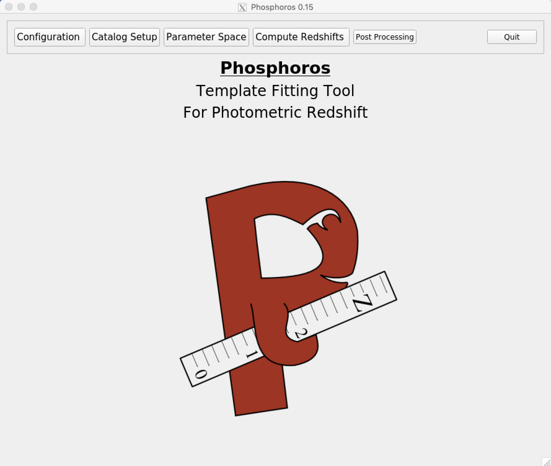
Fig. 2.1 Starting window of the GUI

At the top part of the main window, you can see the navigation menu. This menu is visible at all times, and it allows you to navigate through the different Phosphoros panels.

Note

When launching Phosphoros for the first time, you are asked to download the Phosphoros data package (more details in Phosphoros internal database). Do it! Everything needed to run Phosphoros with the quickstart catalog will be imported (the SED library, the reddening curves, etc.) and located in the proper directory.

In addition, you will be warned that a reference solar spectrum has to be selected for the SED normalization. Navigate to the Configuration --> Aux.Data --> SEDs panel and use the Select button to select the SED named solar_spectrum (as shown in Fig. 2.2).

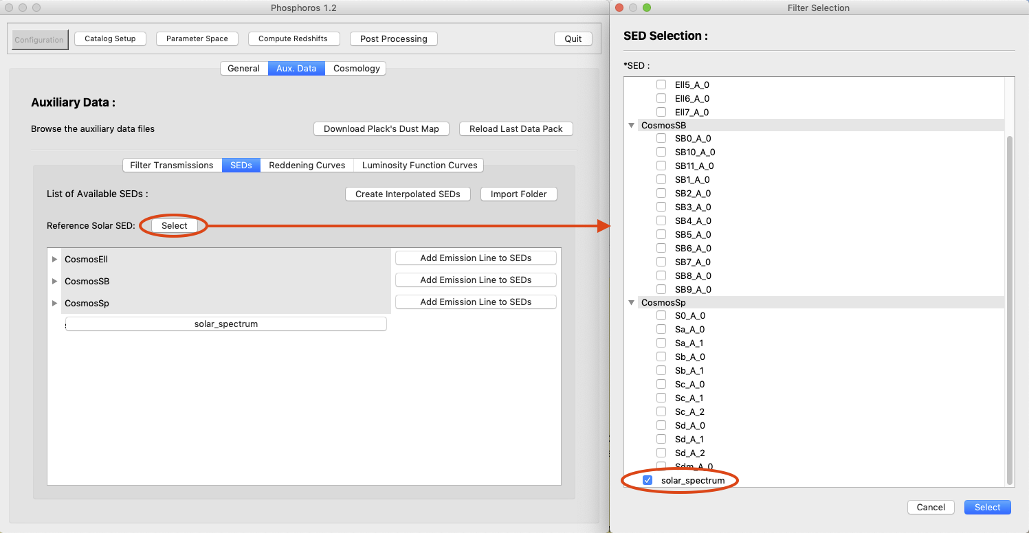
Fig. 2.2 Selecting solar spectrum through the GUI

2.3.1. Filter transmissions

Phosphoros needs the transmission curve of filters to compute modeled photometry. You can see the available filter transmission curves by selecting Filter Transmissions in the Configuration --> Aux.Data panel of the GUI.

Transmission curves are found as files in the directory AuxiliaryData/Filters/Quickstart. Later on this User Manual (Important concepts and data setup) you will learn how to add your own filter transmission curves.

2.4. Examining the input catalog

The quickstart data contain a single catalog file, Catalogs/Quickstart/quickstart.fits. This is an FITS catalog, but Phosphoros can read both ASCII and FITS tables. You can examine the catalog file with your favorite tool (e.g., TOPCAT). It contains photometry for 8 filters, including errors, and a column with spectroscopic redshifts, which can be used for estimating the accuracy of predicted photometric redshifts.

2.4.1. Mapping filters to photometry

Phosphoros needs to know which filter corresponds to the photometry column in the catalog file. This mapping operation is already done for you in the quickstart data (see the red box in Fig. 2.3).

You can see it by selecting Catalog Setup at the navigation menu. You should first select Quickstart from the Catalog drop-down menu, then click the Select File and Import Columns button and select your catalog file. You also have to select the catalog column containing the object ID in the Source ID Column menu.

If you want to plot your results, it is useful to insert the column name containing reference redshifts (here, ZSPEC) in the Reference Z tab.

When you finish you have to click the Save button to persist your modification.

Fig. 2.3 Catalog Setup panel of the GUI. The red box shows the filter mapping for the Quickstart example

Later in the User Manual, you will learn more about how to organize your catalogs (Directory Organization) and how to map columns to filters (GUI: Catalog Setup: Mapping filters to column names).

2.5. Examining the parameter space

During the first step of the template fitting method, Phosphoros builds the photometry for all the models which will be used for the \(\chi^2\) computation. A full explanation of how to define this parameter space is out of the scope of this quickstart tutorial and it will be explained in detail later (GUI: Defining the model parameter space). For the moment, to get an idea how a parameter space looks like, you can select the Parameter Space panel of Phosphoros and select the Quickstart parameter space (see Fig. 2.4).

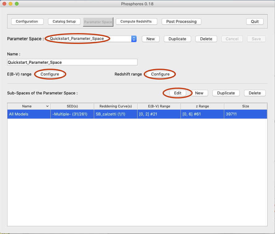
Fig. 2.4 Parameter Space panel of the GUI

Click the Edit button to open the window showing the axes of the parameter space. There you can see that the Cosmos templates are used as SED templates, the Calzetti reddening law is used for the extinction with E_(B-V) in the range 0 to 2 and 0.1 steps, and the redshift is computed for the range 0 to 6, with 0.1 steps.

Note

If the range and the step of redshift and E_(B-V) are not set up yet, you will be asked to do it through the Configure buttons.

2.6. Building the grid of models

So far you had a look of the setup included in the quickstart data pack. Now you are going to use Phosphoros for running the two steps of the template fitting. The execution of them is done in the Compute Redshifts panel of Phosphoros.

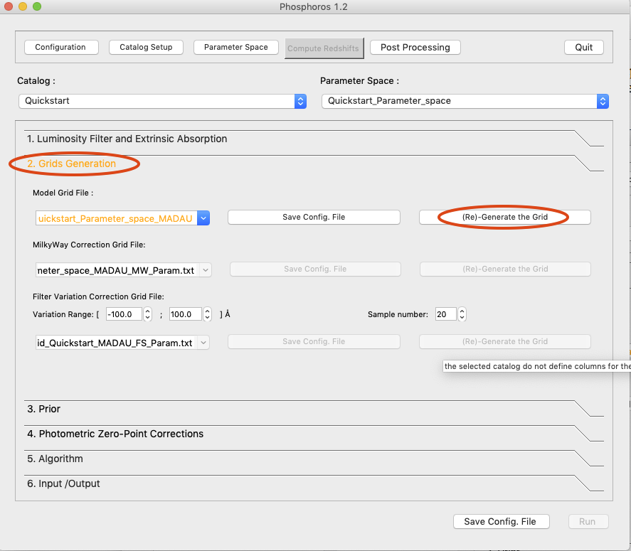
Fig. 2.5 Grid Generation sub-panel inside the Compute Redshift panel of the GUI

This panel contains six collapsable sub-panels, one for each operation you can perform with Phosphoros. The titles of these sub-panels are color-coded, so if you have to take some action in one of them, its title will be presented in orange letters. For example, at the moment we have not performed yet the first step of the model fitting (i.e., computing modeled photometry), so the sub-panel 2. Grids Generation is orange (see Fig. 2.5).

To build the grid of models you just have to click on the 2. Grids Generation label to expand the sub-panel and then click the (Re)-Generate the Grid button. Note that when this operation will finish, the name of the panel will turn black, indicating that you can go on with computing your photometric redshifts.

Tip

When the Save Config. file and/or Run button is grayed out, hover the mouse on it and a tool tip will appear with the list of the missing steps blocking the action.

Note

You do not need to rebuild your modeled photometry, as long as you do not modify your parameter space. Phosphoros will check all the already generated grids of models and, if you already have a compatible one, it will allow you to use it for computing the photometric redshifts.

2.7. Compute photometric redshifts

Now that you have built your models you are ready to compute your first photometric redshifts using Phosphoros! To do that select the 6. Input/Output in the Compute Redshifts panel (Fig. 2.6).

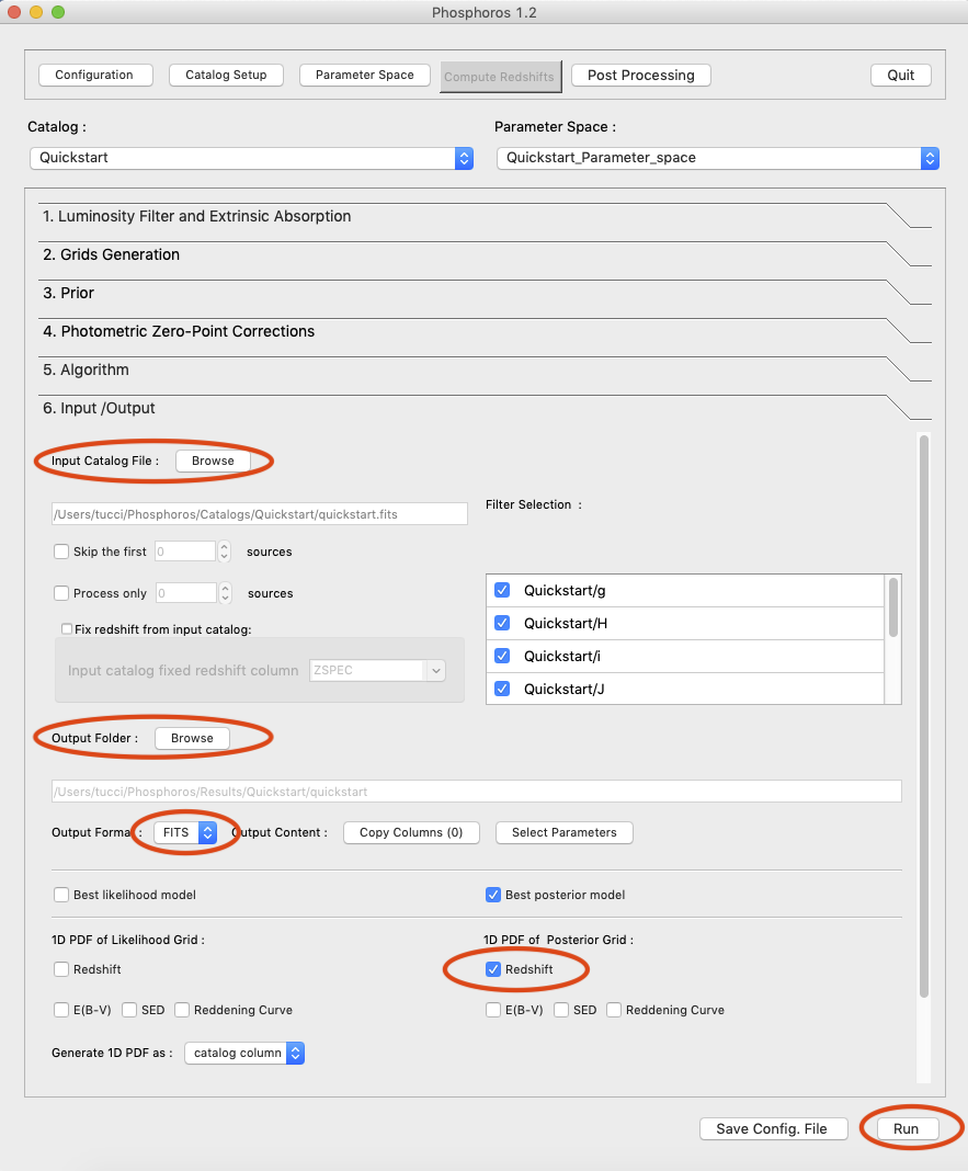
Fig. 2.6 Input/Output sub-panel inside the Compute Redshift panel of the GUI

Here you can setup the input and the output parameters. Note that the catalog included with the quickstart data is already selected as input catalog. Moreover, Phosphoros has already set the output folder for you. This is done based on some rules which should help you to organize your outputs (and avoid overriding them). You can find more details about this organization in Directory Organization. You can however change the output folder to any directory you like. You can also select the format (ASCII or FITS table) of the output catalog.

In the rest of the panel, you can select additional outputs to be produced in the output catalog and directory (best-fit model, 1D PDFs, multi-dimensional distributions, etc). For this tutorial you should select as Output Format FITS and to generate the 1D PDF of the Posterior distribution for Redshift and E(B-V).

Tip

Do not select the multi-dimensional outputs, as this will result in the creation of very big files. These outputs are intended for investigating specific cases, as it is explained later in the User Manual (Posterior Investigation).

To compute the photometric redshifts for your catalog you just have to press the Run button at the bottom right corner of Phosphoros and you are done!

Note

Before estimating redshifts, Phosphoros will compute the weight to be associated to each SED template of the parameter space. This is an optional functionality of Phosphoros. See SED weights for more details.

2.8. Visualizing the results

Even though the output files of Phosphoros can be handled by any software which manages tables (like TOPCAT), Phosphoros provides some post-processing tools to facilitate this process.

The most useful plot for visualizing your results (as long as the input catalog does contain the spectroscopic redshift) is the photoZ-specZ plot. Using this plot you can see how well Phosphoros performed in predicting redshifts.

To see the plot for your results you have to select the Post Processing panel, and click on the Plots button. A pop-up window opens (Fig. 2.7) where you have to provide the path for the catalog with the reference redshifts (e.g., the input catalog if it contains them), the column name of the source ID and of the reference redshifts. However, if the Reference Z column has been declared in the Catalog Setup panel, the input catalog and the corresponding columns are automatically selected.

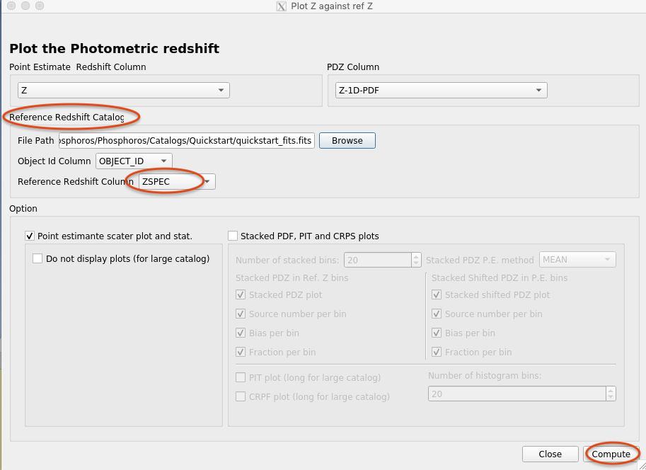
Fig. 2.7 Setup window for the visualization of results with the GUI

Pressing the Compute button will open new windows: the photoZ-specZ plot (Figure 1); the distribution histogram of their relative differences (Figure 2); and the 1D PDF of the model parameters for which the PDF has been computed (e.g., in Fig. 2.8, for redshift and E_(B-V)). At the beginning the 1D PDF plots will be a zero constant line until a source is selected. Colors in the photoZ-specZ plot are associated to the number density of objects, blue at the lowest density and dark red at the highest density.

If you click on a point in the photoZ-specZ plot, you will see at the top left corner the ID of the source, and its redshift and E_(B-V) 1D PDF will be plotted in the corresponding plots.

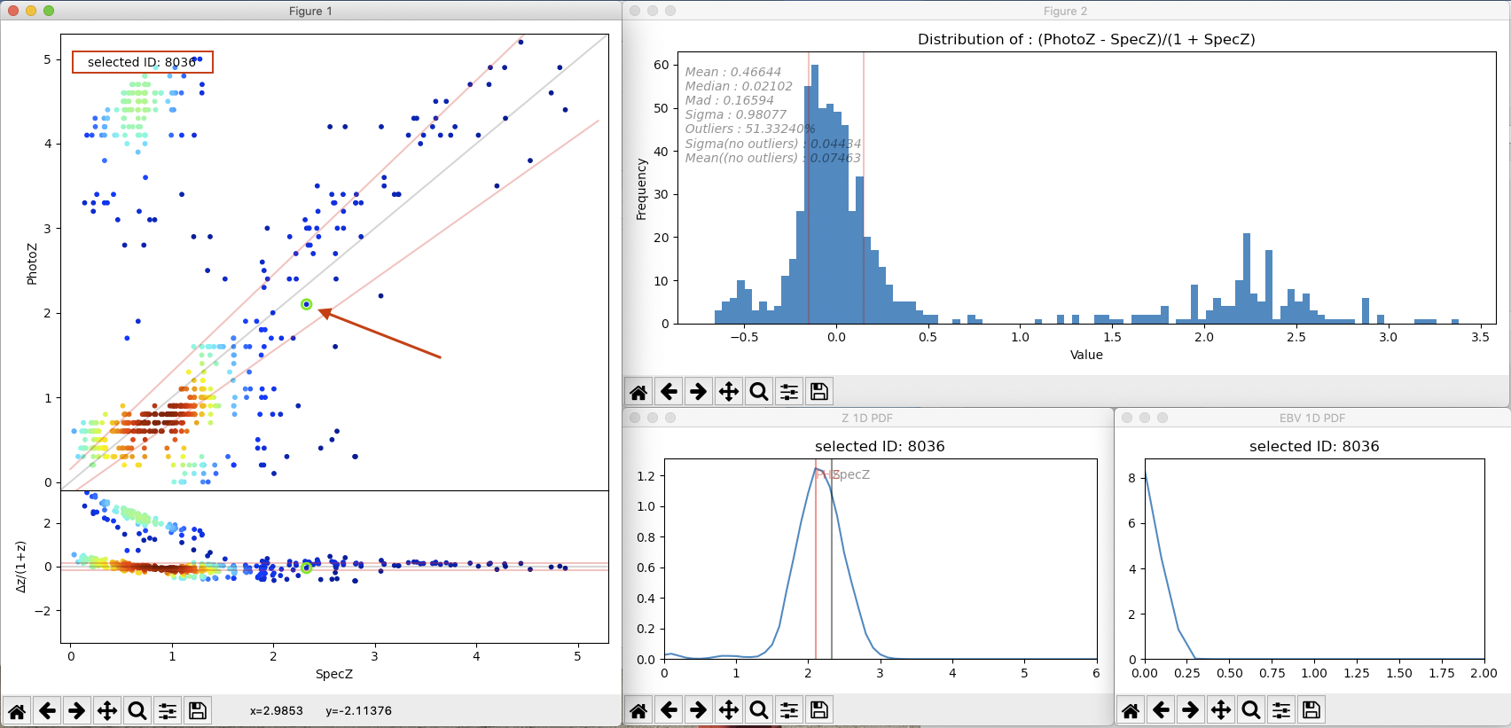
Fig. 2.8 Plots comparing photometric and reference redshifts

Note

These plots are standard matplotlib plots, so some default functionalities (like zooming, etc) are available.

2.9. Summary

During this quickstart tutorial you had a first look of how the Phosphoros GUI works. Phosphoros provides much more advanced options for improving your photometric redshift results, which have not been explain here. The following chapters of the User Manual will navigate you through a more detailed description of how to use Phosphoros and will explain in details all the advanced features, so to achieve optimal photometric redshift estimates.