3.5. Examining results

Output files produced by Phosphoros follow standardized formats (see the Results Format section) and can be handled by any compliant software. Nevertheless, Phosphoros provides some tools to facilitate the process of analysis and visualization of results. In particular:

3.5.1. Statistical Analysis

Phosphoros can compute the following statistical information on the redshift PDF of sources in the output catalog (in brackets, we report the name used in Phosphoros to identify the redshift point estimators; see below):

• Median (Z-1D-PDF_Statistic-MEDIAN)

• Confidence interval at 70, 90 and 95%. This is computed

  1. centering the confidence interval on the mean of the distribution;

  2. taking the confidence interval with the minimum length.

  
  

• For the first two modes of the distribution, the tool finds the best-fitting Gaussian function and computes

  1. the sampled redshift with the highest probability (Z-1D-PDF_Statistic-PHZ_MODE_1_SAMP or Z-1D-PDF_Statistic-PHZ_MODE_2_SAMP);

  2. the mean of the fitted distribution (Z-1D-PDF_Statistic-PHZ_MODE_1_MEAN or Z-1D-PDF_Statistic-PHZ_MODE_2_MEAN);

  3. the redshift at the peak of the fitted distribution (Z-1D-PDF_Statistic-PHZ_MODE_1_FIT or Z-1D-PDF_Statistic-PHZ_MODE_2_FIT);

  4. the area below the fitted distribution.

Warning

The analysis can only be performed if output catalogs contain the redshift PDFs of sources (see the GUI: Computing Redshifts section).

3.5.1.1. Statistical analysis with the GUI

The Post Processing panel in the GUI allows users to apply Phosphoros tools for the statistical analysis of output catalogs (see Fig. 3.12).

Select the catalog type of results to be analyzed (through the Results for Catalog drop-down menu). All the folders belonging to that catalog type and present in the database (below the directory $PHOSPHOROS_ROOT/Results/<Catalog Type>) will appear in the List of processing result.

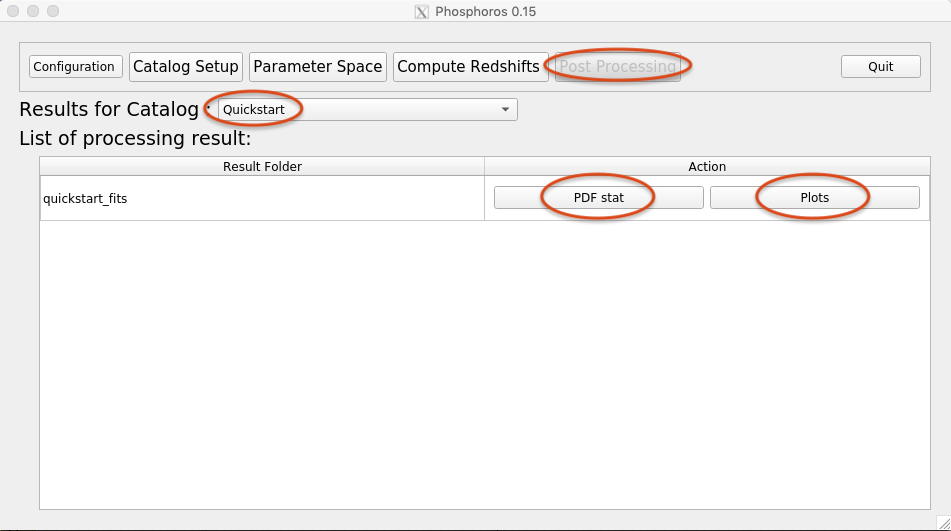
Fig. 3.12 Example of the Post Processing panel in the GUI

Clicking on PDF stat opens a window with the list of statistics that can be computed (see Fig. 3.13). By default, all the possible statistics are selected. Users can deselect those that are not of interest.

The Compute tab at the bottom runs the process. The results are then save in a .FITS file named Z-1D-PDF_Statistic.fits and located in the same directory as the output catalog:

> $PHOSPHOROS_ROOT/Results/<Catalog Type>/<Catalog File Name>/

Fig. 3.13 Window of the GUI with the statistical information that Phosphoros can compute

3.5.1.2. Statistical analysis with the CLI

The process_output_pdz (or POP) action performs the statistical analysis of output catalogs. It calls the ProcessPDF C++ executable and extracts from the redshift PDFs of output catalogs the statistical information described above.

Users have to provide the qualified name of the output catalog by the --input-cat action parameter. For example:

> Phosphoros POP --input-cat=$PHOSPHOROS_ROOT/Results/<Catalog Type>/<Catalog File Name>/phz_cat.fits

The name and the location of the output file (by default out.fits and located in the same directory as the ouput catalog) can be set by the --output-cat option.

The computation of some statistical information can be excluded by the --excluded-output-columns option.

See the full list of options with the usual --help action parameter.

3.5.2. Visualization

Phosphoros provides tools for the visualization of results. In particular, the following plots can be produced:

• A plot comparing photometric redshifts (\(photoZ\)) estimated by Phosphoros with reference redshifts (\(specZ\)) provided by users. Below that, a plot with their relative difference, \((photoZ-specZ)/(1+specZ)\), as a function of \(specZ\) is also shown (left plot in Fig. 3.14). Users can choose among different point estimators of the photometric redshift \(photoZ\) (like the redshift of the best-fit model, the peak of the redshift PDF, and the statical estimators described above in the Statistical Analysis sub-section). Colors in the \(photoZ\,{\rm vs}\,specZ\) plot are associated to the number density of objects, blue at the lowest density and dark red at the highest density.

• The histogram of the relative difference \((photoZ-specZ)/(1+specZ)\). Some basic statistics are computed and shown in the plot (right-top plot in Fig. 3.14).

• The \(photoZ\,{\rm vs}\,specZ\) plot is interactive, and allows users to examine the 1D PDF of model parameters for the sources in the plot (right-bottom plots in Fig. 3.14). By a single click on a source, in fact, its ID will be presented at the top left of the window and all the 1D PDFs that have been computed will be displayed in separated windows, up to eight plots (i.e., the PDF of z, SED, \(E_{B-V}\) and reddening curve for both the likelihood and posterior distribution).

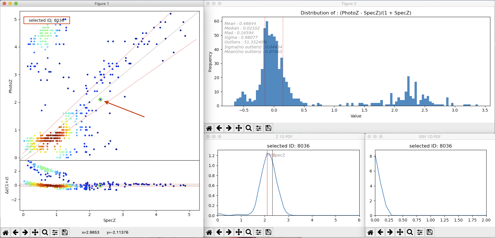
Fig. 3.14 (left) Photometric vs Reference redshifts and their relative difference; (right-top) distribution of the relative difference; (right-bottom) the redshift and \(E(B-V)\) PDF of the selected source in the left plot.

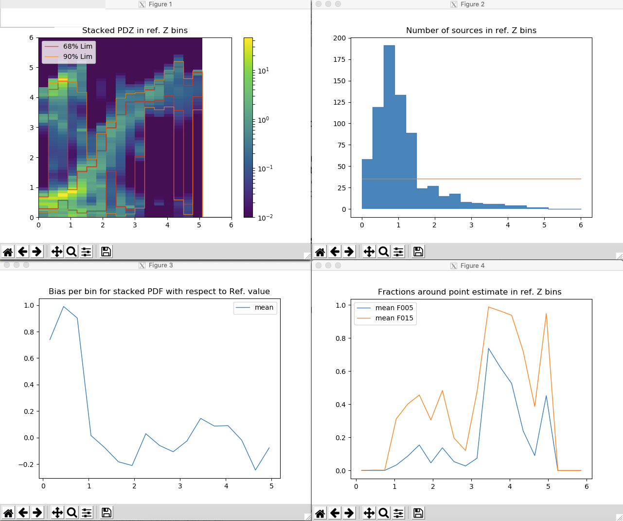
Fig. 3.15 (right-top) Density scatter plot of the stacked PDFs in \(specZ\) bins; (left-top) number sources in \(specZ\) bins; (right-bottom) bias per \(specZ\) bin; (left-bottom) fraction of the stacked PDF around its mean value per \(specZ\) bin.

• A density scatter plot obtained by stacking the redshift PDFs of input sources in reference redshift (\(specZ\)) bins. The contour level at 90% and 68% of the stacked PDFs are also plotted (left-top plot in Fig. 3.15).

• The histogram of the number of sources per \(specZ\) bin (right-top plot in Fig. 3.15).

• The bias of the stacked PDFs with respect to the reference redshifts per \(specZ\) bin (left-bottom plot in Fig. 3.15). In the plot, the bias is computed as difference between the mean of the stacked PDF with the bin center. However, the bias can be also computed using the maximum (MAX), the median (MED) or the fit (FIT) 1 of the stacked PDFs.

• The fractions of the stacked PDFs enclosed in a \(0.05(1+z)\) interval (F005) or in a \(0.15(1+z)\) interval (F015) around the mean of the stacked PDF per \(specZ\) bin (where \(z\) is the center of the bin). As for the bias, the mean can be replaced with the median, the maximum or the fit of the stacked PDF (right-bottom plot in Fig. 3.15).

Note

Similar plots as in Fig. 3.15 can be also generated for shifted redshift PDFs. For each input source, the shifted PDF is obtained by traslating the PDF to have the reference redshift as origin. Again, shifted PDFs are then stacked in redshift bins. In the ideal case, the density scatter should be centered in zero at all redshifts.

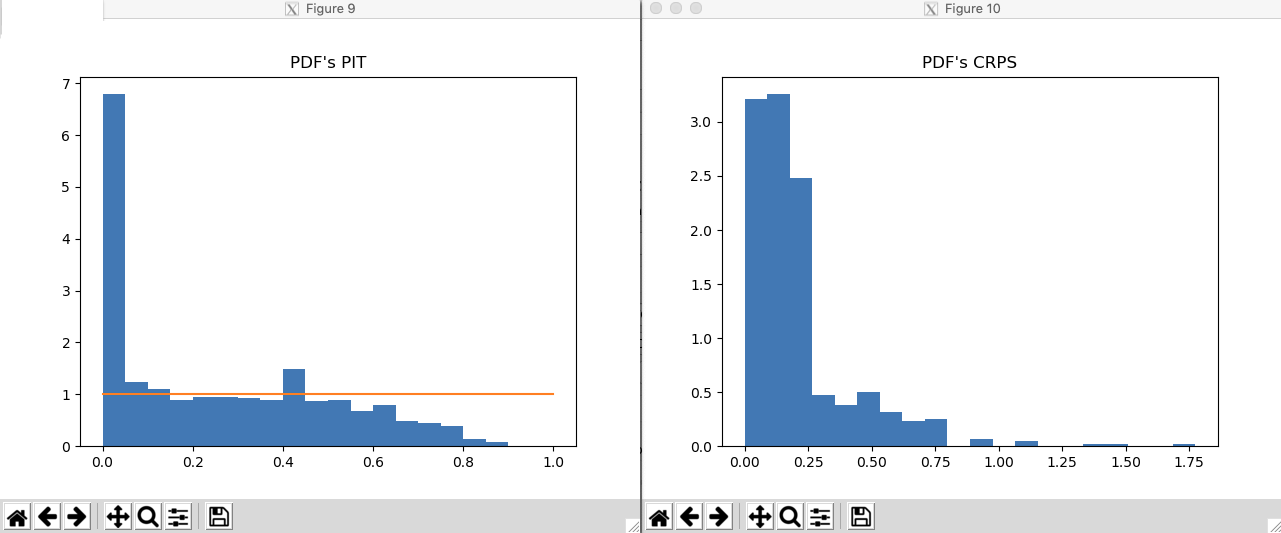
Fig. 3.16 (left) PIT plot; (right) distribution of the CRPS.

In order to assess the performance and the quality of the predicted redshfit PDFs in the output catalog, the following two plots can be also useful (see, e.g., [Hersbach00]; [DIsantoPolsterer18]):

• The Probability Integral Transform (PIT) plot of the redshift PDFs (Left plot in Fig. 3.16).

• The distribution of the Continuous Ranked Probability Score (CRPS) of the redshift PDFs (Right plot in Fig. 3.16).

Warning

The tool to visualize results can be used only for those catalogs for which reference redshifts are known.

Note

All these plots are standard matplotlib plots and come with a navigator toolbar, making available default functionalities like zooming, etc.

Note

Phosphoros also provides a tool for visualizing multi-dimensional likelihoods and posterior distributions. At the moment, it is available only in the CLI. The description of the tool is out of the scope of the Basic Steps chapter. We refer the reader to the Posterior Investigation section.

Fig. 3.17 Post Processing window of the GUI for the visualization of results

3.5.2.1. Visualization with the GUI

The Post Processing panel in the GUI allows users to apply Phosphoros tools for the visualization of results. Clicking on Plots opens a window with the required action parameters (see Fig. 3.17).

By the Point Estimate Redshift Column drop-down menu, different point estimators of the photometric redshift can be selected for the comparison with the reference redshift. They are the redshift associated with the best-fit model (Z), the peak of the redshift PDF (1DPDF-Peak-Z), and all the statistical estimators described in the above Statistical Analysis sub-section.

In Reference Redshift Catalog, users have to select the file where reference redshifts are found, the column name of the source ID and of the reference redshift. However, if a reference redshift column in the input catalog has been provided in the Catalog Setup panel (see the Catalog Setup section), Phosphoros will automatically fill these fields.

In Option users can decide which plots to produce. Clicking on Point estimate scatter plot and stat., Phosphoros will display the plots shown in Fig. 3.14. For very large catalogs, there is the option to not display any plots. Phosphoros will only print basic statistics for the \((photoZ-specZ)/(1+specZ)\) distribution.

Clicking on Stacked PDF, PIT and CRPS plots, users can manually select the plots to display (see Fig. 3.15 and Fig. 3.16 above). By default, all plots but the PIT and CRPS ones are selected. Moreover, plot parameters – such as the number of redshift bins, of histogram bins and the method for the redshift estimate – can be choosen using the corresponding drop-down menus.

The Compute tab at the bottom runs the process and a window per plot opens.

3.5.2.2. Visualization with the CLI

Two different actions are defined for visualization purposes: the plot_specz_comparison (or PSC) action for the plots in Fig. 3.14 and the plot_stacked_pdz (or PSP) action for the plots in Fig. 3.15 and Fig. 3.16.

The PSC action

Users have to provide the directory containing the Phosphoros results by using the --phosphoros-output-dir (or -pod) parameter. The tool itself will automatically detect all the available results in the directory (like 1D PDFs) and it will handle all the possible output formats.

Note

By default, the tool plots the redshift of the best-fit model, i.e. column named Z in the output catalog. If users want to use a different redshift estimator, they should pass the option -pcol=<PHZ column name>. For example, for the redshift corresponding to the peak of the 1D-PDF, the option is -pcol=1DPDF-Peak-Z.

Warning

If users have leftover results from previous executions (e.g., 1D PDFs in separate files), the tool will not recognize that they are belonging to a different run. Therefore the directory should be cleaned before runnning the analysis.

Phosphoros does not copy the reference redshifts in the output catalog. That means that users need to specify the catalog file which contains the reference redshifts. This is done by using the following options:

• --specz-catalog= (or -scat=) the catalog file name, in FITS or ASCII format.

• --specz-cat-id= (or -sid=) the name of the column that contains the source ID (default: ID)

• --specz-column= (or -scol=) the name of the column that contains the reference redshift (default: ZSPEC).

Warning

Phosphoros will use the source ID columns to match the catalog rows of different files. Only rows with matching IDs in all files are plotted by the tool.

Warning

By default, the PSC tool opens new windows and it does not terminate until the windows are closed. The tool is therefore unusable in scripts. If users want to use the tool in a script, they can simply pass the --no-display (or -nd) parameter, which will instruct the tool to only print the statistics on the screen and terminate directly after, without opening any extra windows. In this way, the tool can be run from a script and the standard output streams be parsed to retrieve the statistics.

See the full list of options with the usual --help action parameter. Configuration files can be used through the --config-file option.

The PSP action

Users have to provide the qualified name of the output catalog (in FITS format) containing the redshift PDFs through the --pdz-catalog-file option. The name of the relevant columns inside this file can be specified by the following options:

• --pdz-col-id= the name of the column that contains the source ID (default: ID).

• --pdz-col-pdf= the name of the column containing the redshift PDF (default: Z-1D-PDF).

• --pdz-col-pe= the name of the column containing the redshift estimator. This can be the redshift of best-fit model, Z, or the redshift at the peak of the PDF, 1DPDF-Peak-Z, or one of the redshift estimators discussed in the Statistical Analysis sub-section (default: Z).

Warning

The PSP action is not enabled when output catalogs are in ASCII format or the redshift PDFs are saved in a separated file.

Similarly, there are action parameters for the file containing the reference redshifts:

• --refz-catalog-file= the qualified name of the catalog file including the reference redshifts, in FITS format. If not specified, Phosphoros will look for reference redshifts into the file defined by the --pdz-catalog-file option.

• --refz-col-id= the name of the column that contains the source ID (default: ID).

• --refz-col-ref= the name of the column that contains the reference redshifts (default: Z-TRUE).

Warning

Phosphoros will use the source ID columns to match the catalog rows of the different files. Only rows with matching IDs in all files are plotted by the tool.

The following action parameters concern how to produce the plots:

• --stack-bins= the number of redshift bins for the stacking of the PDFs (default: 20).

• --hist-bins= the number of bins for the histograms in the PIT and CRPS plots (default: 20).

• --stacked-point-estimate= the type of redshift estimate computed from the stacked PDFs. Options are MAX, FIT, MEAN and MED (default: MEAN).

By default, all possible plots will be displayed. In order to disable one of them, it is enough to set the <name>-plot option to False, where the <name> of each plot can be found with the usual --help option. For example, setting --ref-bias-plot=False will disable the bias per redshift bin plot.

3.5.3. Connecting with TOPCAT

The Phosphoros plot_specz_comparison (or PSC) tool is SAMP 2 enabled and it can communicate with a TOPCAT instance. You can enable this functionality by using the parameter -samp. In this case, Phosphoros will search for the first instance of TOPCAT and it will open in it the related catalogs (see Fig. 3.18). From that moment on, all the selections on the plot will be forwarded to TOPCAT and the corresponding rows will be highlighted. The interaction is bidirectional, meaning that if you select a row in TOPCAT, the source will be highlighted in the plot.

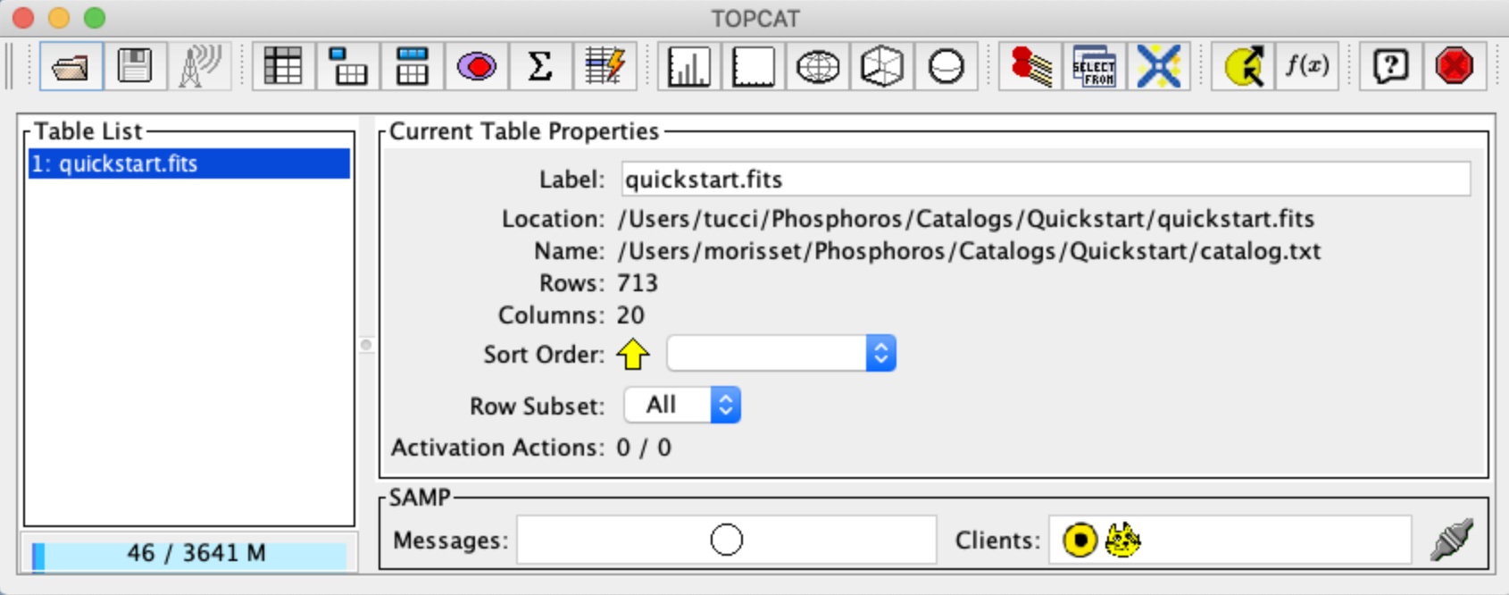
Fig. 3.18 TOPCAT window

Note

If multiple instances of the Phosphoros PSC tool are launched with the SAMP functionality enabled (and connected to the same TOPCAT instance), all selections will be reflected to all the plot windows.

Footnotes

1

In the FIT case, the redshift estimate is computed by fitting the maximum of the stacked PDF by a parabolic function and taking its maximum. This is similar to the MAX estimate but more precise.

2

SAMP, the Simple Application Messaging Protocol, is a messaging protocol that enables astronomy software tools to interoperate and communicate (see, e.g., arXiv:1501.01139).

DIsantoPolsterer18

A. D'Isanto and K. L. Polsterer. Photometric redshift estimation via deep learning. Generalized and pre-classification-less, image based, fully probabilistic redshifts. A&A, 609:A111, Jan 2018. arXiv:1706.02467, doi:10.1051/0004-6361/201731326.

Hersbach00

Hans Hersbach. Decomposition of the Continuous Ranked Probability Score for Ensemble Prediction Systems. Weather and Forecasting, 15(5):559–570, Oct 2000. doi:10.1175/1520-0434(2000)015<0559:DOTCRP>2.0.CO;2.